Tutorial
How StiffStruct works
From an empty screen to a checked, documented analysis in a few minutes. Every step below has a screenshot; click any picture to enlarge it.
The whole workflow in four steps
Choose a structure
Beam, 2D or 3D truss, or 2D or 3D frame. Start blank, from a template, or from a worked example.
Describe it
Geometry, supports, loads and, if you want deflections, a section and a material.
Analyze
Press Ctrl+Enter. The direct stiffness method runs in your browser in milliseconds.
Read, check, export
Diagrams, tables, a printable step-by-step report, and a Python or MATLAB script of the same model.
Getting started
There is nothing to install and no account is needed to build a model. Open the calculator and pick what you want to analyze.
- Open the calculator. It reopens the model you were working on (autosaved in this browser), or starts with a small example beam.
- Choose File → New model… or use the New model… button in Quick actions. You can also open app.html?new=beam directly.
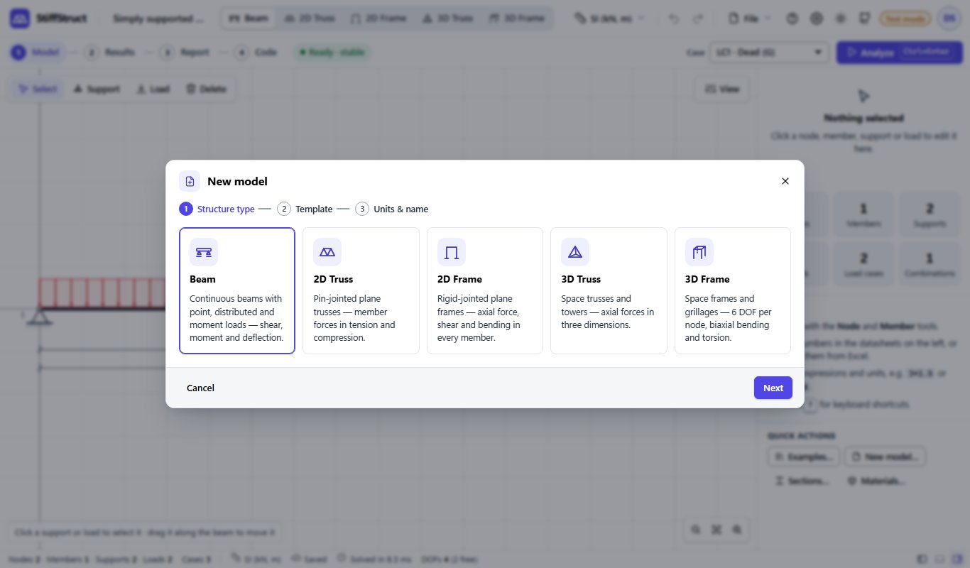
- Pick the structure type.
- Pick a template. Start from a Blank model or from a parametric template (continuous beam, Pratt or Howe truss, portal frame, multi-storey frame, 3D tower…). The preview updates as you change the dimensions.
- Set units and a name, then press Create. You land in the Model step.
Worked examples
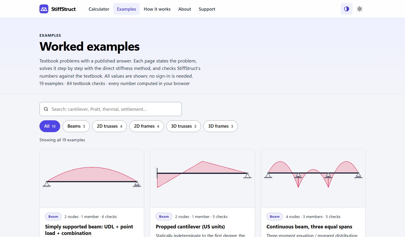
Every example opens on its own page with the problem statement, the data, the figure, the full step-by-step solution and a table that compares StiffStruct with the textbook answer. Press Open in calculator on any card to load it into the editor and change it.
Beam calculator walk-through
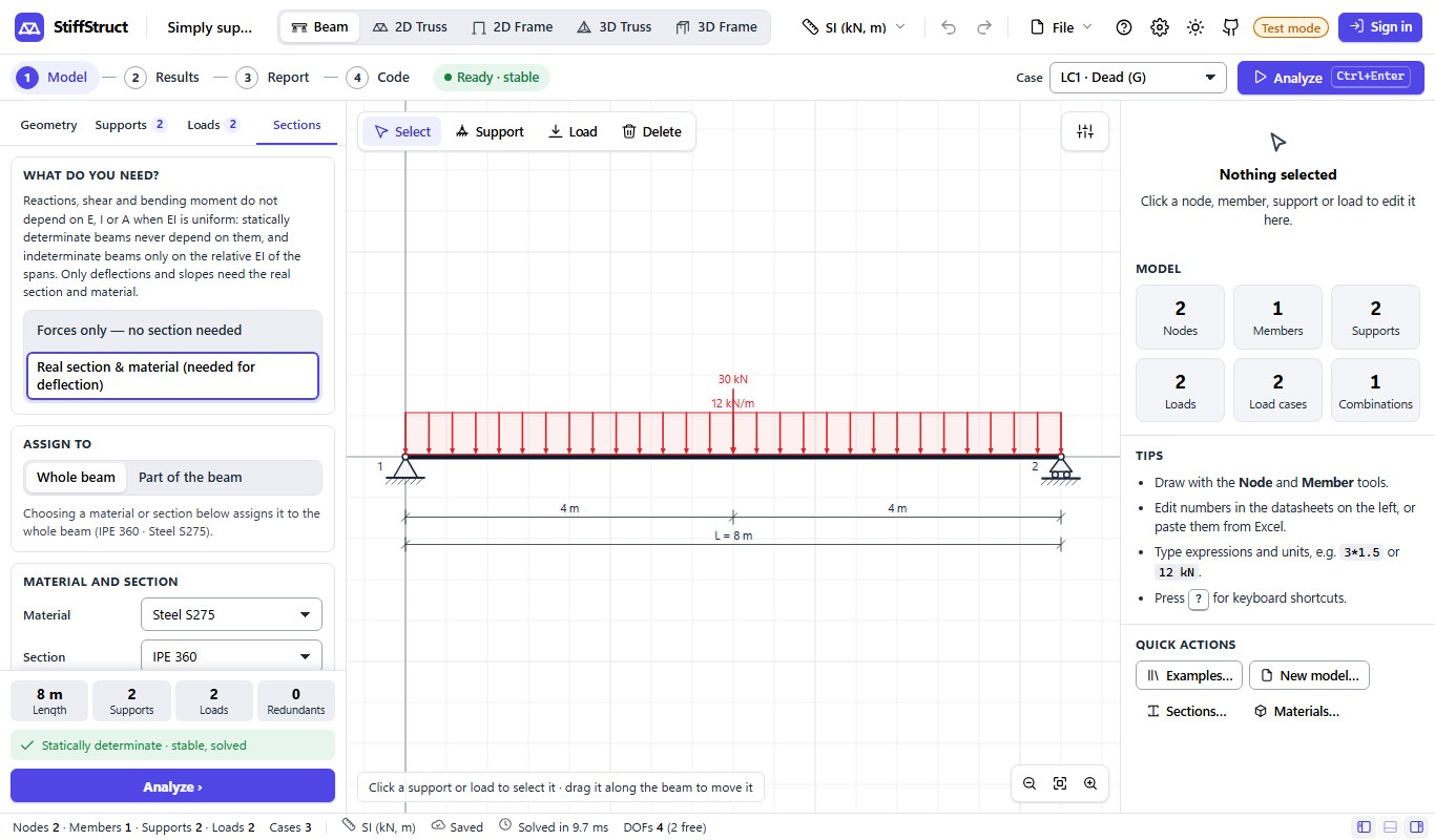
The beam mode is a guided wizard. The four tabs on the left (Geometry, Supports, Loads, Sections) are filled in from left to right, and the picture on the canvas updates after every change.
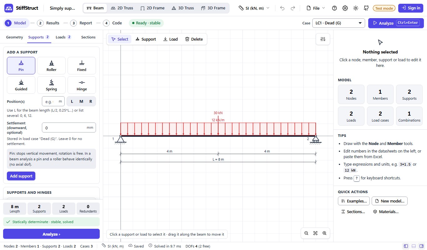
2.1 Geometry and supports
- Geometry. Type the total Beam length. To make a continuous beam, list the span lengths from left to right (for example
4, 6, 4) under Spans. Each span end becomes a joint. - Supports. Choose a type: Pin, Roller, Fixed, Guided, Spring or Hinge (an internal hinge for Gerber beams).
- Position. Type a position or several, such as
0, 6, 12, or use the L M R buttons for the left end, the middle and the right end.Lstands for the beam length, soL/2and0.25*Lalso work. - Press Add support. A Settlement can be added to a support if you need one.
2.2 Loads
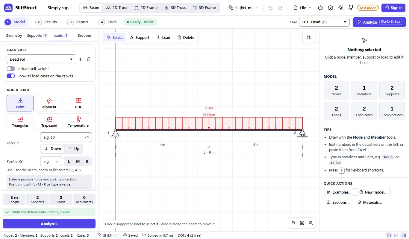
- Pick a load type: Point, Moment, UDL, Triangular, Trapezoid or Temperature (a gradient through the depth).
- Enter the magnitude and direction. Magnitudes are always positive; Down / Up (or CCW / CW for moments) sets the sense. Units follow the unit system you chose; you can also type units, such as
12 kN. - Place it. For a point load give the position. For a distributed load give from and to; leave them empty for the full length.
- Press Add load. Loads appear in the list below the form, where you can edit or delete them, and on the canvas.
- Loads belong to a load case (dead, live, wind…). Pick the case at the top of the tab, or press + to add one. See load cases and combinations.
2.3 Section and material, or forces only
Do you need a section and a material? Only for deflections and slopes.
- Reactions, shear force and bending moment do not depend on E, I or A when the beam has the same stiffness along its length. A statically determinate beam never depends on them; an indeterminate beam depends only on the relative stiffness of its spans.
- Deflection and slope need the real section and material.
- Open the Sections tab and choose Forces only — no section needed if you only want reactions and the shear and moment diagrams. The material and section editors disappear, and the deflection numbers show “needs section”.
- Or choose Real section & material, pick a Material and a Section (search the library of IPE, HEA, HEB, AISC W, HSS and pipe sections, or enter your own properties), and assign it to the whole beam or to part of the beam.
2.4 Analyze and read the results
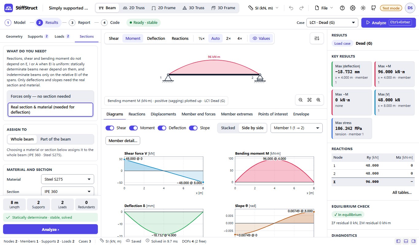
- Press Analyze (Ctrl+Enter). The step bar at the top moves to Results.
- Canvas: switch between Shear, Moment, Deflection and Reactions, change the diagram scale, and turn the value labels on or off.
- Key results (right): largest deflection, positive and negative moment, shear and stress, with the position where each occurs.
- Tables (below the canvas): Reactions, Displacements, Member end forces, Member extremes, Points of interest and, with several load cases, an Envelope.
- Equilibrium check: the sum of the reactions must balance the sum of the loads. StiffStruct shows the residual so that you can see it is zero.
- Use the Case menu at the top right to look at one load case, one combination or the envelope.
2.5 Member detail
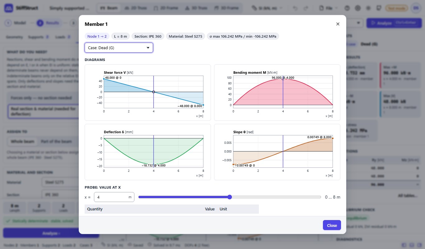
Press Member detail… under the charts for a closer look at one member.
- Four large diagrams: shear V, moment M, deflection δ and slope θ.
- Probe: drag the slider or type a position x to read every quantity at that point.
- The equations of the diagrams along the member and its points of interest.
Trusses and frames
For trusses and frames you work on a drawing canvas and in data tables at the same time. Both always show the same model, so use whichever is faster for the job.
Draw with the tools
The toolbar above the canvas has these tools (the key in brackets selects one):
- Select V
- Node N
- Member M
- Support S
- Load L
- Split X
- Delete D
- Node tool: click to add a node. It snaps to the grid, to other nodes and to members; hold Alt to switch snapping off.
- Member tool: click the start point, then the end point. It keeps chaining from the last point; press Esc to finish.
- Support tool: pick a support type, then click a node.
- Load tool: click a node for a nodal load, or a member for a member load.
- Select tool: click to select, drag empty space to box-select, and drag nodes to move them. The Properties panel on the right edits whatever is selected.
Tables and pasting from Excel
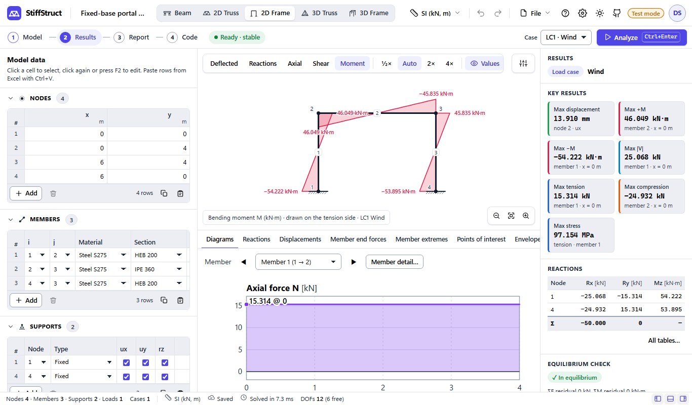
- The left panel lists Nodes, Members, Supports, Loads and Combinations as spreadsheet-like tables.
- Click a cell to select it; click again or press F2 to edit. Cells accept expressions and units, such as
3*1.5or12 kN. - Paste rows from Excel with Ctrl+V. Copy a block of cells in your spreadsheet, select the first cell here and paste. Add appends a row; the copy and paste buttons under each table move whole tables.
Supports and member loads
- Supports: pin, roller, fixed, or custom restraints per degree of freedom (tick ux, uy, rz…). Springs, inclined rollers and prescribed settlements are available.
- Member loads: point and distributed loads, in global or local axes, plus temperature and fabrication-error loads.
- Releases: mark a member end as pinned (for example a truss bar inside a frame) with the release columns, or tick Truss for an axial-only bar.
3D models
3D trusses and 3D frames use the same tables and the same workflow; the canvas becomes a 3D viewer.
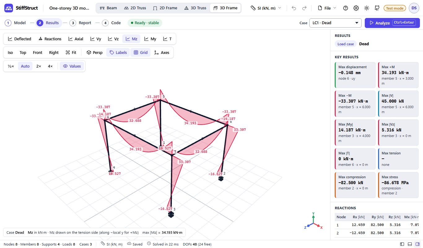
- Move around: drag to orbit, right-drag to pan, use the wheel to zoom. The buttons Iso, Top, Front, Right and Fit set a view, and Persp switches between perspective and orthographic.
- Add nodes by clicking the ground grid (a dialog lets you type X, Y and Z), or type coordinates in the Nodes table. Join them with the Member tool.
- Local axes: a 3D frame member has its own axes, and a roll angle rotates the section about the member axis. Bending is resolved about both axes.
- Results: choose Deflected, Reactions, Axial, Vy, Vz, Mz, My or T (torsion) to draw that quantity on every member.
Units
Pick the unit system once; every input and every result follows it. Nothing is hard-coded.
- Click the unit button in the header (for example SI (kN, m)) and choose a system, or choose Custom… to set a unit for each quantity separately.
- You can change units at any time. All values are stored in SI internally, so changing the display never changes a result.
- You can also type units in any field (
12 kN,3 ft,250 mm). A number without a unit is read in the current display unit.
| Preset | Force | Length | Typical use |
|---|---|---|---|
| SI (kN, m) | kN | m | Most textbooks and codes |
| SI (kN, mm) | kN | mm | Small steel and timber members |
| MKS (tf, m) | tf | m | Regions that use tonne-force |
| US (kip, ft) | kip | ft | US practice, long spans |
| US (kip, in) | kip | in | US practice, sections and plates |
Load cases and combinations
A load case is a set of loads that act together (dead load, live load, wind). A combination adds cases with factors, such as 1.35 G + 1.5 Q.
- Add a case. In the beam wizard use the + next to the load case selector; in the other modes use the load case table. Give it a name and a category (dead, live, wind, snow, temperature…).
- Add loads to the active case. New loads go into the case that is selected. Tick Include self-weight to add the weight of the members to a case (this needs a section and a material).
- Create combinations. Open the Combinations table. Add a row and type a factor for each case, or press Generate… to create the combinations of a design code.
- Read the results. The Case menu at the top right switches between a single case, a combination and the Envelope of everything, which shows the largest and smallest value at every position.
The step-by-step report
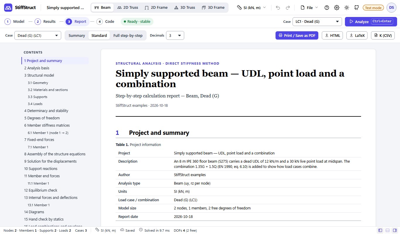
The Report step writes the whole calculation as a document: every matrix, every vector and every check, with the numbers of your model.
- Press Report in the step bar. The contents list on the left jumps to any section.
- Detail: Summary (results only), Standard or Full step-by-step (every member stiffness matrix, the assembly, the solution and the hand check).
- Case and Decimals choose which load case or combination is reported and how many digits are printed.
- Export: Print / Save as PDF opens the print dialog (choose “Save as PDF” as the printer), HTML downloads a standalone page, LaTeX downloads the source for your own document, and K (CSV) downloads the stiffness matrix.
Code export
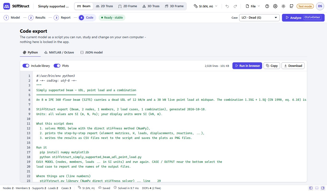
The Code step turns the current model into a script you can read, run and change. The numbers in the script are the same as in the app.
- Press Code in the step bar and choose a tab: Python, MATLAB / Octave or JSON model.
- Include library puts the whole solver into the file so it runs on its own. Plots adds the diagrams.
- Run in browser runs the Python script on the page, with nothing to install, and shows its printed report and plots. The first run downloads the Python runtime (Pyodide) once from a public CDN, so it needs an internet connection.
- Copy or Download the file, then run it on your computer:
pip install numpy matplotlib, thenpython the_file.py. The script prints the step-by-step report and writes CSV files and PNG plots next to it.
Free sign-up: why values need an account
Building a model and seeing the shape of the result is always free. A free account unlocks the numbers.
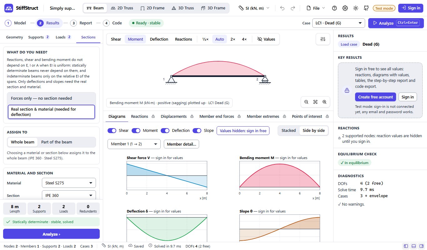
- Before you sign in you can draw the structure, add loads and press Analyze. You see the shape of the shear force, bending moment and deflection diagrams.
- To see the values (reactions, extremes, tables, the step-by-step report and the code export), choose Sign in in the header or the card in the results panel, then Create free account.
- Sign up with an e-mail address and a password, or continue with Google. The account is free and needs no payment details; it shows the diagram shapes. To see the values (reactions, diagram values, tables), start the 3-day free trial of Student or Pro.
- After signing in, the screen updates at once. You stay signed in on this device until you choose Sign out from the account menu.
Saving and sharing
Your work is kept on your device. The File menu in the header has everything you need to keep it or pass it on.
- Autosave: the model is saved in this browser after every change (the status bar shows Saved). It is never uploaded. Clearing your browser data removes it.
- Save JSON / Open JSON: download the model as a small file and open it later or on another computer. Ctrl+S saves.
- Copy share link: the model travels inside the link, so anyone who opens it gets a copy. Nothing is stored on a server.
- Project info: add a title, description, author and project number; they appear in the report.
- Undo and redo: every edit can be undone with Ctrl+Z.
- Settings: the gear icon sets the number of decimals, the theme (auto, light or dark) and the text contrast. The same choices apply on every page of this site.
Open a model from a link
These addresses start the calculator in a given state, which is handy for teaching and for bookmarks:
app.html?new=beamstarts a new beam (alsotruss2d,frame2d,truss3d,frame3d).app.html?example=frame-portal-lateralopens a worked example.- Add
&mode=results,&mode=reportor&mode=codeto jump to that step.
Ready to try it?
Open the calculator and have a beam analyzed in a couple of minutes, or read a worked example first.